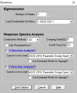
The dynamic analysis calculates the modes and frequencies of vibration for the model. This is a prerequisite to the response spectra analysis, which uses these frequencies to calculate forces, stresses and deflections in the model. For more information, see Dynamic Analysis - Response Spectra.
The process used to calculate the modes is called an eigensolution. The frequencies and mode shapes are referred to as eigenvalues and eigenvectors. Refer to the Program Limits section for information on the maximum number of modes that can be solved for in RISA. The program can also solve for an approximate type of eigenmode called a Ritz Vector.
The dynamic analysis uses a lumped mass
matrix with inertial terms. Any vertical loads that exist in the
Load Combination for Mass will
be automatically converted to masses based on the acceleration of gravity
entry on the Solution tab of the Model Settings. However, you must
always enter the inertial terms
as
To Perform a Dynamic Analysis / Eigensolution
Note
You may specify how many of the model’s modes (and frequencies) are to be calculated. The typical requirement is that when you perform the response spectra analysis (RSA), at least 90% of the model's mass must participate in the solution. Mass participation is discussed in the Response Spectra Analysis topic.
The catch is you first have to do a dynamic analysis in order to know how much mass is participating so this becomes a trial and error process. First pick an arbitrary number of modes (5 to 10 is usually a good starting point) and solve the RSA. If you have less than 90% mass, you'll need to increase the number of modes and try again. Keep in mind that the more modes you request, the longer the dynamic solution will take.
Note
The eigensolution is based on the stiffness characteristics of your model and also on the mass distribution in your model. There must be mass assigned to be able to perform the dynamic analysis. Mass may be calculated automatically from your loads or defined directly.
In order to calculate the amount and location of the mass contained in your model, RISA takes the vertical loads contained in the load combination you specify for mass and converts them using the acceleration of gravity defined in the Model Settings. The masses are lumped at the joints and applied in both global directions (X and, Y ).
You may also specify
mass directly. This option allows you to restrict the mass to a
direction. You can also apply a mass moment of inertia to account
for the rotational inertia effects for distributed masses.
Note
The eigensolution procedure for dynamic analysis is iterative, i.e. a guess is made at the answer and then improved upon until the guess from one iteration closely matches the guess from the previous iteration. The tolerance value is specified in the Model Settings and indicates how close a guess needs to be to consider the solution to be converged. The default value of .001 means the frequencies from the previous cycle have to be within .001 Hz of the next guess frequencies for the solution to be converged. You should not have to change this value unless you require a more accurate solution (more accurate than .001?). Also, if you're doing a preliminary analysis, you may wish to relax this tolerance to speed up the eigensolution. If you get warning 2019 (missed frequencies) try using a more stringent convergence tolerance (increase the exponent value for the tolerance).
After you’ve done the dynamic solution, you can save that solution to file to be recalled and used later.
Note
When you request a certain number of modes for dynamic analysis (let's call that number N), RISA tries to solve for just a few extra modes. Once the solution is complete, RISA goes back to check that the modes it solved for are indeed the N lowest modes. If they aren't, one or more modes were missed and an error is reported.
Dynamics modeling can be quite a bit different than static modeling. A static analysis will almost always give you some sort of solution, whereas you are not guaranteed that a dynamics analysis will converge to a solution. This is due in part to the iterative nature of the dynamics solution method, as well as the fact that dynamics solutions are far less forgiving of modeling sloppiness than are static solutions. In particular, the way you model your loads for a static analysis can be very different than the way you model your mass for a dynamic analysis.
The term “dynamics solution” is used to mean the solution of the free vibration problem of a structure, where we hope to obtain frequencies and mode shapes as the results.
In general, the trick to a “good” dynamics solution is to model the structure stiffness and mass with “enough” accuracy to get good overall results, but not to include so much detail that it take hours of computer run time and pages of extra output to get those results. Frame problems are simpler to model than those that include plate elements. “Building type” problems, where the mass is considered lumped at the stories are much easier to successfully model than say a cylindrical water tank with distributed mass. It is often helpful to define a load combination just for your dynamic mass case, separate from your “Dead Load” static case (You can call it “Seismic Mass”). Your seismic mass load combination will often be modeled very differently from your “Dead Load” static case.
Modes for discretized mass models with very few degrees of freedom may not be found by the solver, even if you know you are asking for fewer modes than actually exist. In this case it may be helpful to include the self weight of the model with a very small factor (i.e. 0.001) to help the solver identify the modes.
Distributed
mass models with plate elements, like water tanks, often require
special consideration. You will want to use a fine enough mesh of
finite elements to get good stiffness results. Often though,
the mesh required to obtain an accurate stiffness will be too dense to
simply model the mass with self-weight or surface loads. You will
want to calculate the water weight and tank self-weight and apply it in
a more discrete pattern than you would get using surface loads or self-weight.
This method of using fewer
Whenever you perform a dynamic analysis of a shear wall structure, and the walls are connected to a floor, you must be careful to use a fine mesh of finite elements for each wall. Each wall should be at least 4 elements high between floors. This will give you at least 3 free joints between them.
When you perform
a dynamic analysis of beam structures, such that you are trying to capture
the flexural vibrations, (i.e., the beams are vibrating vertically or
in the transverse direction), you must make sure that you have at least
3 free joints along the member between the points of support. If
you use a distributed load as the mass, you must remember that some of
the load will automatically go into the supports and be “lost” to the
dynamic solution. In general, you will get the best results by applying
your mass as joint loads to the free
The mass of the structure that has not been activated by the solved number of periodic modes may still be included in the response spectra analysis results. This is done by checking the Calc. Residual Mass box. This checkbox calculates a residual mass mode shape which helps to show where the missing mass in the structure is located. It also includes the response of this missing mass as a static correction to the response spectra results. The acceleration used to calculate this static correction vector is based on largest acceleration from the specified response spectra which occurs between the user entered Cut Off frequency (see below) and the zero period acceleration.
Note:
If you apply your dynamic mass with distributed loads or surface loads on members/plates that are adjacent to supports, remember that the some of the load will go directly into the support and be lost to a traditional dynamic solution. The mass that can actually vibrate freely is your “active mass”, as opposed to your “static mass” which includes the mass lost into the supports. If you are having trouble getting 90% mass participation, you should roughly calculate the amount of mass that is being lost into your support to determine if that is the cause of the problem.
Since this mass is directly associated with boundary conditions and cannot be activated by a traditional eigensolution mode, it is referred to as the Residual Rigid Response of the structure. The common solution to account for this response, is to check the Calc. Residual Mass? checkbox. This will calculate a "Missing Mass Vector" or "Residual Mass Vector" to account for this residual mass in the dynamic analysis.
Alternatively, one may switch to the Ritz Vector dynamic solver because Ritz modes inherently include correction for the rigid response
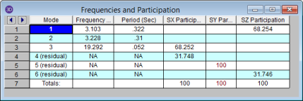
Access the Frequencies and Participation spreadsheet by selecting Frequencies from the Results Menu.
 Analysis_files/image008.jpg)
These are the calculated model frequencies and periods. The period is simply the reciprocal of the frequency. These values will be used along with the mode shapes when a response spectra analysis is performed. The first frequency with a high participation is sometimes referred to as the model's natural or fundamental frequency. These frequency values, as well as the mode shapes, will be saved and remain valid unless you change the model data, at which time they will be cleared and you need to re-solve the dynamics to get them back.
Also listed on this spreadsheet are the participation factors for each mode for each global direction, along with the total participation. If the participation factors are shown in red (as opposed to black) then the response spectra analysis (RSA) has not been performed for that direction. If the RSA has been done but a particular mode has no participation factor listed, that mode shape is not participating in that direction. This usually is because the mode shape represents movement in a direction orthogonal to the direction of application of the spectra. See Dynamic Analysis - Response Spectra for more information.
Note:
Access the Mode Shape spreadsheet by selecting Mode Shapes from the Results Menu.
 Analysis_files/image012.jpg)
These are the model's mode shapes. Mode shapes have no units and represent only the movement of the nodes relative to each other. The mode shape values can be multiplied or divided by any value and still be valid, so long as they retain their value relative to each other. To view higher or lower modes you may select them from the drop-down list of modes on the Window Toolbar.
Note
These mode shapes are used with the frequencies to perform a Response Spectra Analysis. The first mode is sometimes referred to as the natural or fundamental mode of the model. The frequency and mode shape values will be saved until you change your model data. When the model is modified, these results are cleared and you will need to re-solve the model to get them back.
 Analysis_files/image016.jpg)
You can plot and
animate the mode shape of the model by
A common problem you may encounter are “localized modes”. These are modes where only a small part of the model is vibrating and the rest of the model is not. Localized modes are not immediately obvious from looking at the frequency or numeric mode shape results, but they can be spotted pretty easily using the mode shape animation feature. Just plot the mode shape and animate it. If only a small part of the model is moving, this is probably a localized mode.
The problem with localized modes is that they can make it difficult to get enough mass participation in the response spectra analysis (RSA), since these local modes don’t usually have much mass associated with them. This will show up if you do an RSA with a substantial number of modes but get very little or no mass participation. This would indicate that the modes being used in the RSA are localized modes.
Quite often, localized modes are due to modeling errors (erroneous boundary conditions, members not attached to plates correctly, etc.). If you have localized modes in your model, always try a Model Merge before you do anything else. See Model Merge for more information.